All Transit

Interactive map

Transit connects the densest cities but is also surprisingly prevalent in some remote Western states. I wanted to find and display all these routes. Once I'd done that for the U.S., why not the world? This project visualizes data from the Transitland project. The name alludes to All Streets.

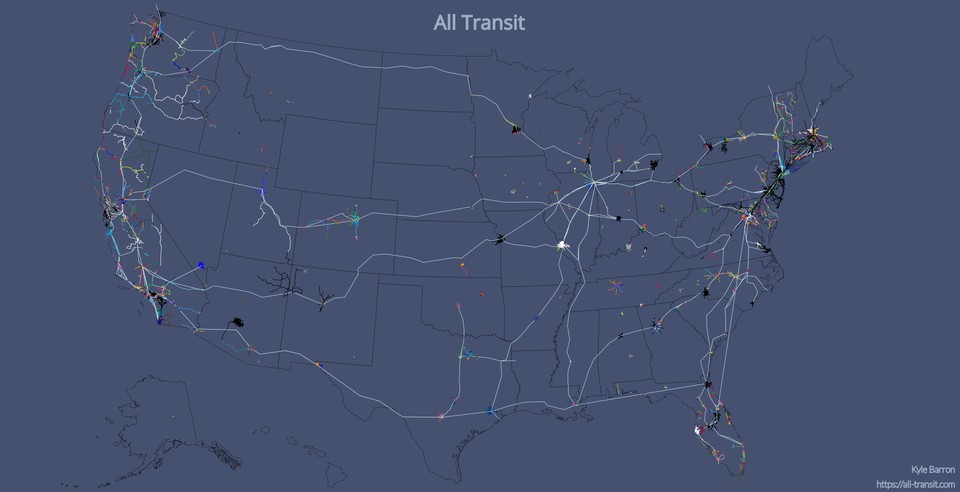
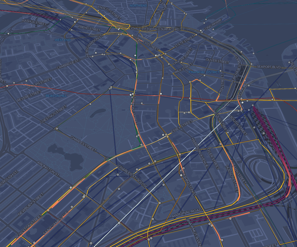
The schedule animation is my favorite part of the project. If you zoom into a city (currently U.S. only) you can see streaks moving around that correspond to transit vehicles: trains, buses, ferries. This data takes actual schedule information from the Transitland API and matches it to route geometries.

This rest of this blog post gives an overview of how the map is made.

Transitland

I use the Transitland project as my data source, which compiles GTFS feeds from around the world, and harmonizes the data into a single dataset. You can read more about why that's important here.

Transitland serves static transit information; it does not currently support GTFS real time feeds (but could in the future). Their data model is split into five components: Operators, Routes, RouteStopPatterns, Stops, and ScheduleStopPatterns.

An operator is a transit agency that offers services to the general public along fixed routes. A route contains all information about a single transit service as defined by the transit agency. A route can be a bit of a nebulous topic, since often a single name has several branches. A RouteStopPattern decomposes each route into a single linear geometry. A route can be defined by one or many RouteStopPatterns. A stop is each point along a route or RouteStopPattern where passengers may get on or off. A ScheduleStopPattern contains schedule information for each individual edge of the route. So if a route has 10 stops in a line, there will be 9 ScheduleStopPattern data points for each transit service scheduled along that route.

Download

Currently, Transitland doesn't offer bulk downloads. In order to download all the data I had to find the best way to find and store all the data through their API endpoints, which they have for each of the five categories enumerated above.

Each of API endpoint allows for a geographic bounding box. At first, I tried to just pass a bounding box of the entire United States to each endpoint and download results a page at a time. Unsurprisingly, that method isn't successful for the endpoints that have more data to return, like stops and schedules, because each API request has a timeout of 120 seconds, and it takes a while to find and return the unindexed one-millionth row in a database. [^1]

[^1]:

It might be possible to use the database indexes better by providing the min_id query parameter.

Because of this, I found it best in general to split API queries into smaller pieces, by using e.g. operator or route identifiers. I ended up downloading routes, route stop patterns, and stops by operator and schedule data by route. I wrote a Python/CLI wrapper for accessing the Transitland database, to help with providing geometries and paging through all results.

N.B. I currently am hosting bulk downloads of the data I collected for the project. You can find appropriate links on the About page of the project.

Data Analysis

Most of the data-generating code for this project is done in Bash, jq, GNU Parallel, SQLite, and a couple Python scripts. In general, data is kept in newline-delimited JSON and newline-delimited GeoJSON for all intermediate steps to facilitate streaming and keep memory use low. However, I found that the schedule data was large enough to necessitate transitioning to SQLite.

Operator, route, and stop information is encoded into Mapbox Vector Tiles using Tippecanoe. I use jq to reshape the source GeoJSON to keep only necessary attributes of each Feature.

Schedule data

Schedule data from Transitland doesn't have a geometric component. In order to connect schedules to geometries, you need to match the schedule data to the routes and stops data.

If you match schedule data just to routes, you have no way of knowing where along the route the two stops are, and if you match schedule data just to stops, you have no knowledge of the geometry between those two points.

Since some schedule data is missing links to route stop patterns, I first tried to use just the routes data. For each schedule stop pair, I found the Point geometries of its start and end stops, found the nearest points on the route for each of those stops, and retrieved the geometry between those two stops.

This can be problematic, however, because routes can have complex geometries. For example, metro lines in Chicago might be represented geometrically as a loop; starting in the suburbs, going downtown around The Loop, and back to the suburbs. When I use this process to match the schedule stop pair to the route, I sometimes match one stop to the first end of the route, and the other stop to the other end of the route. This caused my program to think that the train went to downtown Chicago and back in one minute, and the animation looked haywire depicting a train moving through Chicago at 600 miles per hour.

Helpfully, most (though not all) schedule data is also linked to a route stop pattern, and the schedule data also generally has linear referencing distances along that route stop pattern. So for example, a schedule stop pair might say that the origin stop is 100 (meters) along the route stop pattern's geometry and that the destination stop is 900 (meters) along its geometry. This allows for a much more accurate way of finding schedule geometries. I take the route stop pattern, project it into a local coordinate system with units in meters (I use the local UTM zone), and then cut the route stop pattern's LineString geometry using those two distances using Shapely's linear referencing methods.

Once I have a geometry for that schedule, I linearly interpolate timestamps along each coordinate between start and end. I export this data as GeoJSON Features, where each geometry is a LineString with three-dimensional coordinates: longitude, latitude, and time.

Schedule tiles

Now that I have these three-dimensional geometries, I need to figure out the best way to transport them to the client. Unfortunately, at this time Tippecanoe doesn't support three-dimensional coordinates. The recommendation in that thread was to reformat to have individual points with properties. That would make it harder to associate the points to lines, however.

I decided to go with a custom data format; essentially tiled, gzipped, minified, JSON. Since I know that all features are LineStrings, and since I have no properties that I care about, I keep only the line's coordinates. The verbose depiction of the data the client receives:

Copycopy code to clipboard
[
    // First LineString
    [
        // Coordinate of LineString
        [
            0, 1, 2
        ],
        // Coordinate of LineString
        [
            1, 2, 3
        ]
    ],
    // Second LineString
    [
        []
        ...
    ]
]

In order to make the data download manageable, I cut each JSON into xyz map tiles, so that only data pertaining to the current viewport is loaded. For dense cities with high frequency transit like Washington DC and New York City, some tiles can still be quite large. I cut the schedule tiles into full resolution at zoom 13, and then generate overview tiles for lower zooms that contain a fraction of the features of their child tiles.

Website

All portions of the website are self-hosted. The website itself is static and hosted on Github Pages. The map tiles come from OpenMapTiles and are served with mbtileserver on a Google Cloud f1-micro instance. I have map tiles set to cache through Cloudflare to hopefully cope fine with any spikes in demand. Vector tiles with operator, route, and stop information are also hosted on the Google Cloud instance. The JSON tiles I use for the schedule animation are currently hosted on AWS S3.

The website is coded with React and JavaScript, using Gatsby as the static site generator. I use React Map GL/Mapbox GL JS for rendering the basemap and the routes layer. I use Deck.gl's TripsLayer on top for rendering the schedule animation.

Performance

Although performance still isn't as good as I'd like on lower-powered and mobile devices, it's better than where I started.

Minimize data downloads

The source data for routes and especially for schedule information is huge. In order to serve this data over a web map, they need to be compressed and sliced into smaller pieces to download. This is why map tiling exists.

I use Mapbox Vector Tiles for transmitting operator, route, and stop data to the client. Vector tiles are great because they're highly compressible, and really easy to create with Tippecanoe.

In order to keep the size of the vector tiles small, the stops layer is omitted until zoom 11, and the routes layer omits metadata about the stops on each route until zoom 11. (The maximum zoom level of data in the vector tiles is 11, but the data will display past zoom 11 thanks to overzooming.)

Unfortunately, Tippecanoe only supports 2D data at this time. This means that I had to develop my own solution for getting the schedule data to the client, because I need a third dimension on those geometries (longitude, latitude, time). For the time being I've settled on tiled, gzipped, minified, JSON. Since I know that all schedule data are LineStrings, I keep only the geometry part of the GeoJSON, and don't transmit any properties data about each Feature to the client.

Since I couldn't use Tippecanoe for generating these JSON tiles, I developed my own workflow for cutting GeoJSON features into tiles. I chose a reasonably high zoom level, 13, which contains all schedule data in the selected time period in full resolution. For lower zooms, I take a random fraction of a tile's children tiles to keep tile sizes reasonable.

Minimize data updates

I render invisble operator service area polygons so that I can easily find the operators whose service area is in the viewbox. However I've found that constantly updating the list of nearby operators when panning can impact performance, so instead I only compute that list when the operators option panel is open.

I also turn off the schedule animation when the current zoom is below the minimum zoom at which I show the animation. I'm not sure how much this helps performance because the Deck.gl TileLayer already is invisble below that zoom threshold, but it can't hurt.

Deck.gl optimizations

Deck.gl has a page in its documentation detailing strategies for improving performance.

I set useDevicePixels to false. When true, this prop tells Deck.gl to render at double the resolution on a high DPI display, which means that it must do 4x the pixel computations. When the animation is more important than the crispness of the map rendering, set this to false.

I also attempted to use precomputed binary attributes but hit some errors and decided it wasn't worth it to debug right now. In the future I'd like to figure out how to use binary data directly.